CS184 Summer 2025 Homework 1 Write-Up
Link to webpage: https://cs184.snoopboopsnoop.com/
GitHub Repository: https://github.com/cal-cs184/hw-rasterizer-jcheng
Overview
In Homework 1, we built working functions for triangle rasterization that utilize supersampling for more accurate results, SVG transformations, barycentric coordinates, and both pixel sampling for texture mapping and level sampling using mipmap levels.
The most interesting thing I learned is how barycentric coordinates allow the interpolation of values smoothly inside a triangle with color specifically. This reminded me of color theory and spectral hues commonly used in digital design color gradient palettes. By using barycentric coordinates to interpolate three vertex colors that we have often defined in class as red, green, and blue, we have recreated gradient tools that mix RGB in software such as Photoshop. Dragging around the color is adjacent to moving the point P inside a triangle in barycentric coordinates and shows how we can smoothly move along a continuous color spectrum. Every pixel can be treated as a weighted average of the colors at the endpoints or corners, just like the rasterizer we created in Task 4. -Crystal
I learned a lot through the process of implementing the things we discussed in class. Many of the topics that I didn't feel quite comfortable with, like the rasterization pipeline, became clearer as I had to trace through and make changes to it in task 2. One of my main objectives in taking this course is to better understand the terms in my modded Minecraft shader settings, and through this homework I was exposed to "antialiasing" and "mipmaps". -Walter
Task 1: Drawing Single-Color Triangles
Rasterizing a triangle is the process of taking a continuous triangle (defined by 3 vertices in some space, for Homework 1 this is a 2D plane of some width and height) and writing its shape to a screen.
Since most computer graphics are shown using raster displays, meaning the display is some array of pixels, this means we need to pick a set of pixels to color that best matches the actual triangle.
For this task we're keeping it simple: take the center of each pixel; if the point lands within the triangle, color it in. If not, don't.
Our Rasterization Algorithm
Given floats x0, y0, x1, y1, x2, y2 and a Color object color, this is how we rasterize it:
1. Get the Bounding Box
The top-left and bottom-right corners of the bounding box around a triangle are simply the minimum and maximum x and y values out of the three vertices:
// bounding box coordinates
Vector2D boxmin(floor(min({ x0, x1, x2 })), floor(min({ y0, y1, y2 })));
Vector2D boxmax(floor(max({ x0, x1, x2 })), floor(max({ y0, y1, y2 })));
2. Force CCW Winding Order & Vectorize Everything
First thing we'll do is check that the vertices were passed in CCW order; this is important for the inside() function.
As was shown in Discussion 2, winding order can be checked by picking a vertex to be the origin and taking the cross product of the
vectors formed by the other 2 vertices:
Vector2D v1(x1 - x0, y1 - y0);
Vector2D v2(x2 - x0, y2 - y0);

// store vectors around triangle CCW (using cross product)
if (cross(v1, v2) < 0) {
	float tempX = x1;
	float tempY = y1;
	x1 = x2;
	y1 = y2;
	x2 = tempX;
	y2 = tempY;
}
Since these are 2D vectors, their cross product will be a scalar, which will tell us the winding direction: If it's negative (CW winding order) we want to switch the points.
For convenience we compute vectors representing the edge of the triangles (see below for inside()).
array<Vector2D, 6> edges = {
	Vector2D(x1 - x0, y1 - y0),
	Vector2D(x0, y0),
	Vector2D(x2 - x1, y2 - y1),
	Vector2D(x1, y1),
	Vector2D(x0 - x2, y0 - y2),
	Vector2D(x2, y2),
};
3. Iterate Over Pixels & Check If Inside Triangle
We iterate over all pixels in the bounding box.
How is your algorithm no worse than one that checks each sample within the bounding box of the triangle?
Easy: our algorithm is the one that checks each sample within the bounding box of the triangle!
for (int x = boxmin.x; x <= boxmax.x; x++) {
	for (int y = boxmin.y; y <= boxmax.y; y++) {
		...
	}
}
Quick check to make sure we're even on the screen,
for (int x = boxmin.x; x <= boxmax.x; x++) {
	for (int y = boxmin.y; y <= boxmax.y; y++) {
		if (x < 0 || x >= width || y < 0 || y >= height) {
			continue;
		}
		...
	}
}
(note: I actually forgot to do this until way later in this assignment, like after finishing Task 6, and it was causing segmentation faults and weird rendering artifacts until I realized I was trying to render in pixels that weren't on the screen)
Then check if our pixel is inside the triangle, using the inside() function. If it is, then draw it.
for (int x = boxmin.x; x <= boxmax.x; x++) {
	for (int y = boxmin.y; y <= boxmax.y; y++) {
		if (x < 0 || x >= width || y < 0 || y >= height) {
			continue;
		}
		if (inside(Vector2D(x, y), edges)) {
			fill_pixel(x, y, color);
		}
	}
}
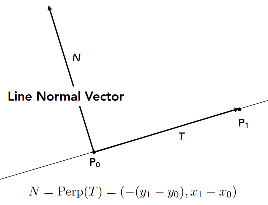
The inside() Function
inside() takes a point v, represented as a 2D vector, and an array of 2D vectors that we consider in pairs:
the first index gives the edge from vertices Pi to Pi+1, and the second gives the vertex Pi.
bool inside(const Vector2D& v, const array<Vector2D, 6>& edges) {
	for (int i = 0; i < edges.size(); i+=2) {
		Vector2D T = edges.at(i);
		Vector2D V = v - edges.at(i + 1);
		Vector2D N(-T.y, T.x); // normal to T

		if (dot(V, N) < 0) return false;
	}
	return true;
}
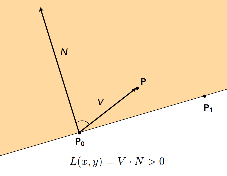
We consider each vertex of the triangle (the for loop) and construct vectors
T, N, and V as shown in the figures below. Then, the
dot product \(V \cdot N\) tells you if V is inside or outside the line. In this case,
if the dot product is negative, then we know it is outside. Repeat for all 3 edges and if V
is within all of them then you know you're inside the triangle.
Note: If the vertices were in clockwise winding order, the normal vector would be pointing outside of the triangle, so we'd have to negate everything. That's why we check for winding order in step 2.
|
|
inside(), and an example dot product.
Since point P is "inside" the triangle (one edge of it), the dot product is positive.
(Lecture 2 Slides, Ren Ng)
Can you show a png screenshot of basic/test4.svg with the default viewing parameters and
with the pixel inspector centered on an interesting part of the scene?
Task 2: Antialiasing by Supersampling
To fix our little aliasing problem, we have implemented supersampling, an intuitive but inefficient form of antialiasing.
Our Supersampling Algorithm, Data Structures, and Rasterization Pipeline Changes
1. Alter Sample Buffer Array
The first thing we did was alter some functions in the rasterization pipeline to support supersampling.
Like the HW 1 spec suggests, this includes RasterizerImp::set_sample_rate() and
RasterizerImp::set_framebuffer_target().
In both functions, this was the original line for resizing the sample buffer:
this->sample_buffer.resize(width * height, Color::White);
We changed it to
this->sample_buffer.resize(width * height * sample_rate, Color::White);
Why? In the rasterization pipeline, the sample buffer is a C++ vector that stores sampling data in the form of
Color objects. Originally, for single-pixel sampling, this was a vector of size width * height,
meaning each index corresponded to a pixel on screen. In fact, in the original RasterizerImp::resolve_to_framebuffer(),
the function simply took each index of RasterizerImp::sample_buffer and converted the Color into
its RGB (0-255) components and stored them in the corresponding place in the framebuffer:
for (int k = 0; k < 3; ++k) {
    this->rgb_framebuffer_target[3 * (y * width + x) + k] = (&col.r)[k] * 255;
}
But when supersampling, each pixel now contains sample_rate samples, which means the sample buffer needs
to be scaled appropriately.
2. Fix RasterizerImp::fill_pixel()
Before we touch supersampling the triangle, we need to fix the way fill_pixel()
works to support the new sample_buffer size. Originally, it just put the Color
parameter c directly into the sample buffer at its corresponding (x,y) index,
sample_buffer[y * width + x] = c;
but now that we have scaled the sample buffer up we need to change this slightly. Plus, the intuition gained from fixing this function will help during triangle rasterization.
void RasterizerImp::fill_pixel(size_t x, size_t y, Color c) {
// NOTE: You are not required to implement proper supersampling for points and lines
// It is sufficient to use the same color for all supersamples of a pixel for points and lines (not triangles)
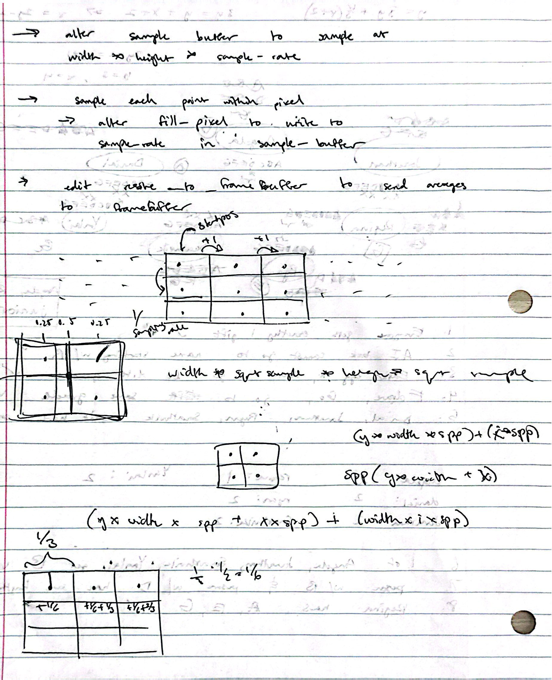
// I did this ^^ -Walter
int dp = sqrt(sample_rate); // samples per unit direction
int startPos = (y * width * sample_rate) + (x * dp); // position of top left sample
for (int i = 0; i < dp; ++i) {
for (int j = 0; j < dp; ++j) {
// fill dp x dp box with color c in sample_buffer
int buffer_pos = startPos + (j * width * dp) + i;
sample_buffer[buffer_pos] = c;
}
}
}
Let's break down the code above. We know we have sample_rate samples per pixel, and we can assume
this number is a square so the length and width of the sample space inside of a pixel is simply
int dp = sqrt(sample_rate); // samples per unit direction
From this, we can get the index of the top-left sample in our pixel (x,y) in the sample buffer, which I call startPos.
We want to be at pixel row y. Each row in the sample buffer has width width * dp, and the row we want
will be at y * dp. Additionally, once we have found the start of the yth row, we need to move over to our
x position at x * dp. This looks like:
int startPos = (y * width * sample_rate) + (x * dp); // position of top left sample
Now we can iterate through all sample_rate subpixels and give them all the same color,
since we don't have to supersample lines and points. Using the nested for iterators
i, j, the position of subpixel (i,j) in the sample buffer was calculated similar to above.
int buffer_pos = startPos + (j * width * dp) + i;
So I had some trouble figuring out how to traverse the sample buffer properly (see above).
After I took some time to read through rasterizer.cpp/h and the Task 2 spec
it probably only took me around 15 minutes to write the code for it, however I then had to spend
an additional hour debugging because I had the math wrong for indexing subpixels, but I didn't know that
so I thought there was some problem with other parts of my code until I finally realized that I was off by
a factor of dp in the indexing formula. I think God saw my Task 1 code run perfectly first try
and decided that I needed some retribution.
3. Supersampling Triangle Rasterization
Now that we've figured out indexing this part is easy. We're using mostly the same code as Task 1 in
RasterizerImp::rasterize_triangle() but we now need to check multiple points inside each pixel
instead of just 1. Originally, we simply checked if the center of the pixel was in the triangle:
if (inside(Vector2D(x + 0.5, y + 0.5), edges)) {
	fill_pixel(x, y, color);
}
But now we want to split the pixel into sample_rate subpixels and sample at their centers.
This is done with the same code as in step 2 with fill_pixel(), but with the introduction
of some additional variables dx, offset.
int dp = sqrt(sample_rate);
float dx = 1.0f / dp; // length of sample
float offset = dx / 2; // dist to center of sample

for (int i = 0; i < dp; ++i) {
	for (int j = 0; j < dp; ++j) {
		int startPos = (y * width * sample_rate) + (x * dp);

		if (inside(Vector2D(x + offset + i * dx, y + offset + j * dx), edges)) {
			sample_buffer[startPos + (j * width * dp) + i] = color;
		}
	}
}
These two variables are used to get the center point of each subpixel (see figure below).
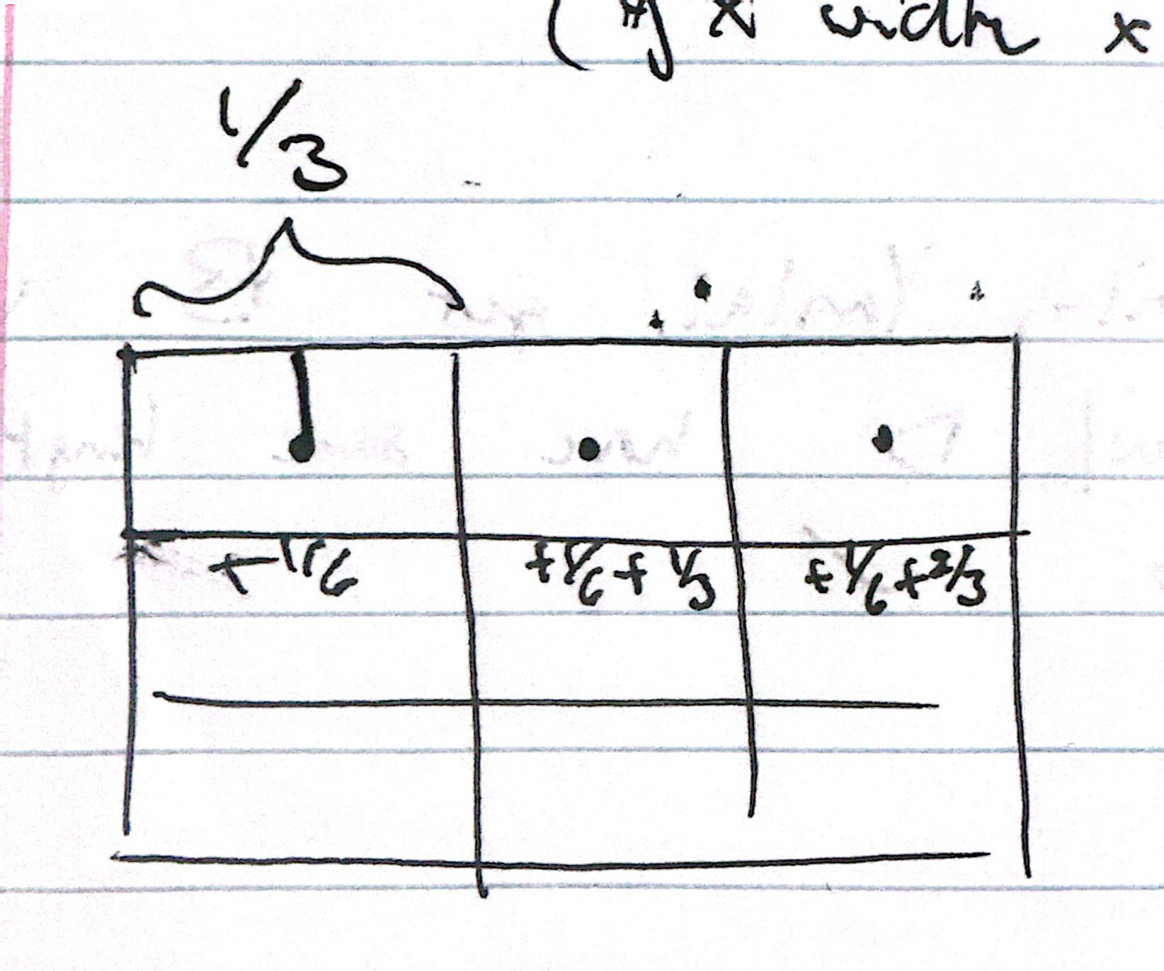
sample_rate = 9, dx = 1/3, offset = 1/6
4. Downsample to Framebuffer
It's looking good, we have correct sample buffers now, but the RasterizerImp::resolve_to_framebuffer()
function does not know how to handle our scaled sample buffer! To resolve this, we'll take all the color values in a
pixel and average them out, effectively downsampling the subpixels into a single pixel once more.
Again, we'll use the same indexing formula from step 2/3.
void RasterizerImp::resolve_to_framebuffer() {
	for (int x = 0; x < width; ++x) {
		 for (int y = 0; y < height; ++y) {
		int dp = sqrt(sample_rate);
		int startPos = (y * width * sample_rate) + (x * dp);

		// sum color of all samples
		Color col;
		for (int i = 0; i < dp; ++i) {
			for (int j = 0; j < dp; ++j) {
				col += sample_buffer[startPos + (j * width * dp) + i];
			}
		}
		col *= (1.0f / sample_rate); // average color

		for (int k = 0; k < 3; ++k) {
			this->rgb_framebuffer_target[3 * (y * width + x) + k] = (&col.r)[k] * 255;
		}
	}
}
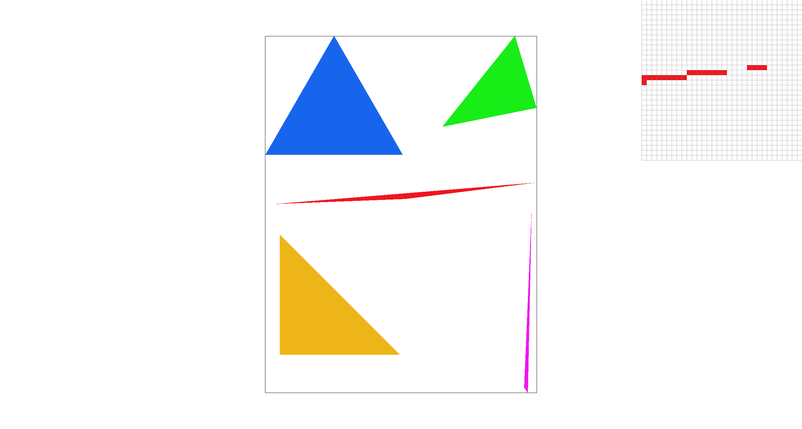
Can you show png screenshots of basic/test4.svg with the default viewing parameters and sample
rates 1, 4, and 16 to compare them side-by-side?

sample_rate=1 |

sample_rate=4 |
sample_rate=16 |
There is a very noticeable difference between the rasterizations at different sample rates. This is because for very acute corners like this one, with single-pixel sampling there is a high chance that the triangle lands within the pixel, but only through the top/bottom half. With higher and higher sampling rates, you get a more accurate approximation of what is or isn't in the pixel, at the cost of exponential computation. Additionally, downsampling creates a blurred effect along the lines of the triangles, which removes jaggies and artifacts (like seen at sample rate 1).
Why is supersampling useful?
Supersampling is extremely useful to prevent aliasing, reducing jaggies, the artifacts that appear as jagged pixelated edges when images on rendered normally. Using only the center as the one sample per pixel results in harsh transitions between two pixels that could have drastically different information stored within them. Supersampling obtains more data that smooths out these jaggies to blend results from multiple subpixels. The result is much closer to the real image.
Man, I really miss when we were doing those dot products in Task 1. Can we do some more linear algebra?
Task 3: Transforms
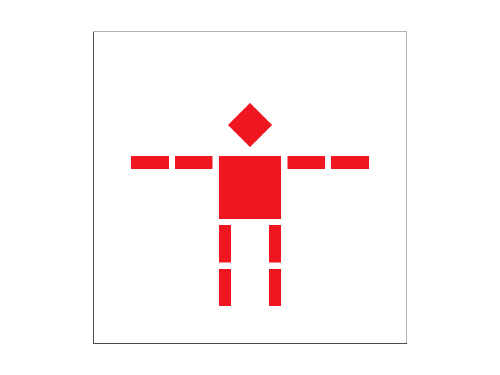
We were given 3 empty basic 2D transformation matrix functions and asked to fill them in for translation, scaling, and rotation. These operations change the position, size, and orientation of geometric shapes they are applied to. In this task, we connected these transformation functions to the given robot.svg, allowing us to draw its head, torso, arms, and legs.
The Transform Functions
Translate(dx, dy)
Translation creates a matrix that shifts the geometric shape that it is applied to by dx units horizontally
and dy units vertically.
Function's Code:
Matrix3x3 translate(float dx, float dy) {
	// row0
	float a = 1, b = 0, c = dx;
	// row1
	float d = 0, e = 1, f = dy;
	// row2
	float g = 0, h = 0, i = 1;
	return Matrix3x3(a, b, c, d, e, f, g, h, i);
}
Scale(sx, sy)
Scaling a geometric shape scales that object by sx in the x-direction and
sy in the y-direction. Objects as a result can increase or decrease in size according to whether the
values are above or below 1.
Function's Code:
Matrix3x3 scale(float sx, float sy) {
	// row 0
	float a = sx, b = 0, c = 0;
	// row 1
	float d = 0, e = sy, f = 0;
	// row 2
	float g = 0, h = 0, i = 1;

	return Matrix3x3(a, b, c, d, e, f, g, h, i);
}
Rotate(deg)
The rotate function constructs a matrix that rotates a point or shape around the origin by an angle given in degrees as the input of the function. The matrix uses the standard rotation form rotating counterclockwise since we use positive angles in a right-handed coordinate system.
Function's Code:
// The input argument is in degrees counterclockwise
Matrix3x3 rotate(float deg) {
	float rad = deg * PI / 180;
	float co = cos(rad);
	float si = sin(rad);

	// row0
	float a = co, b = -si, c = 0;
	// row1
	float d = si, e = co, f = 0;
	// row2
	float g = 0, h = 0, i = 1;

	return Matrix3x3(a, b, c, d, e, f, g, h, i);
}
Matrix multiplication shows how linear algebra directly affects graphics by manipulating its visual elements. Understanding the values in these transformation matrices can allow us to better master different orientations of shapes.
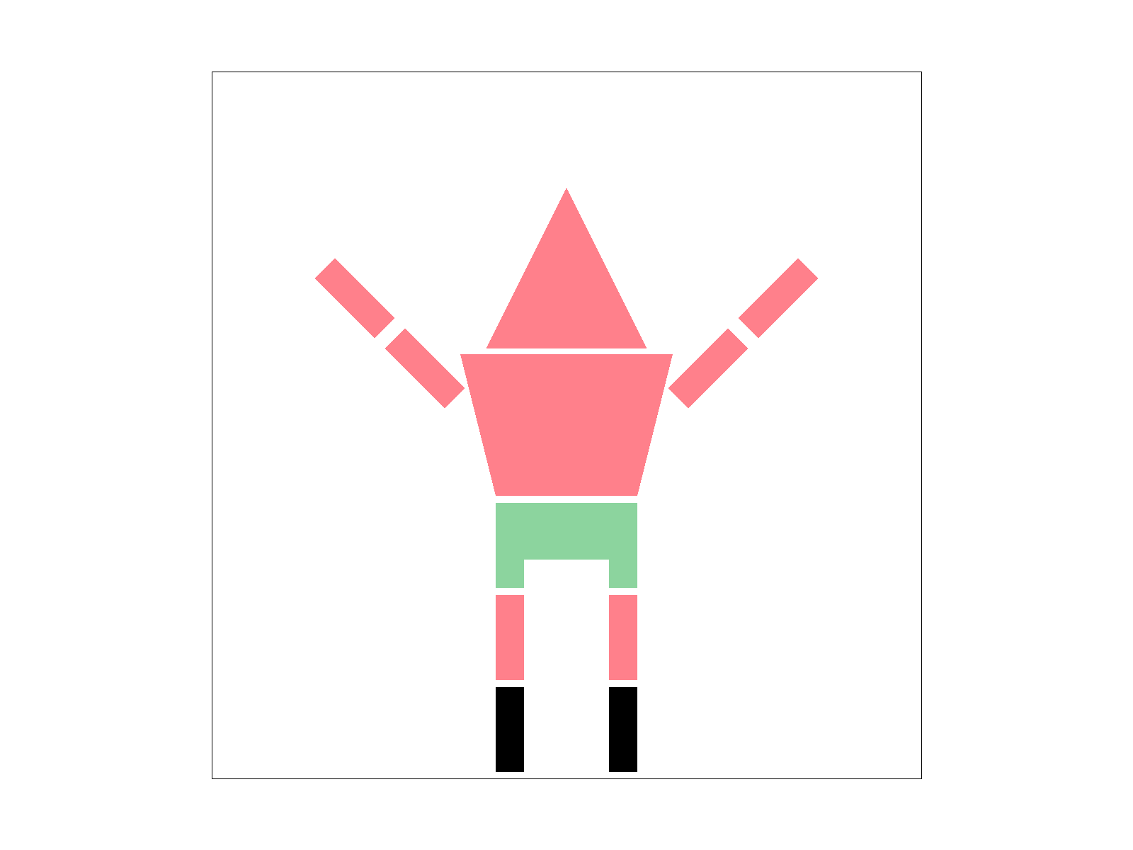
Create an updated version of svg/transforms/robot.svg with cubeman doing something more interesting, like waving or running. Feel free to change his colors or proportions to suit your creativity. Save your svg file as my_robot.svg in your docs/ directory and show a png screenshot of your rendered drawing in your write-up.
To create Patrick from Spongebob Squarepants with black high heels and long legs in a cheering pose, I first customized the colors of the shapes to the exact pink and green hex values. Then, I changed the points given in the polygon fill for his torso to construct a trapezoidal body shape. Using the translate and rotate function, I shifted his arms outwards to create distance from his now scaled up torso. His arms were then rotated 45 and -45 degrees each to make his arms into a cheering position. In order to get the effect of pants, I added a new geometric shape, using the translate function to place it at coordinates right below his torso. Lastly to extend his legs, I added a third geometric shape, translating the entire leg section to the negative y-direction.
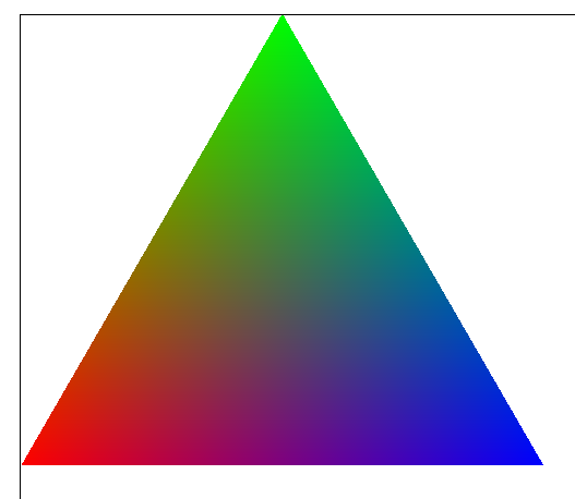
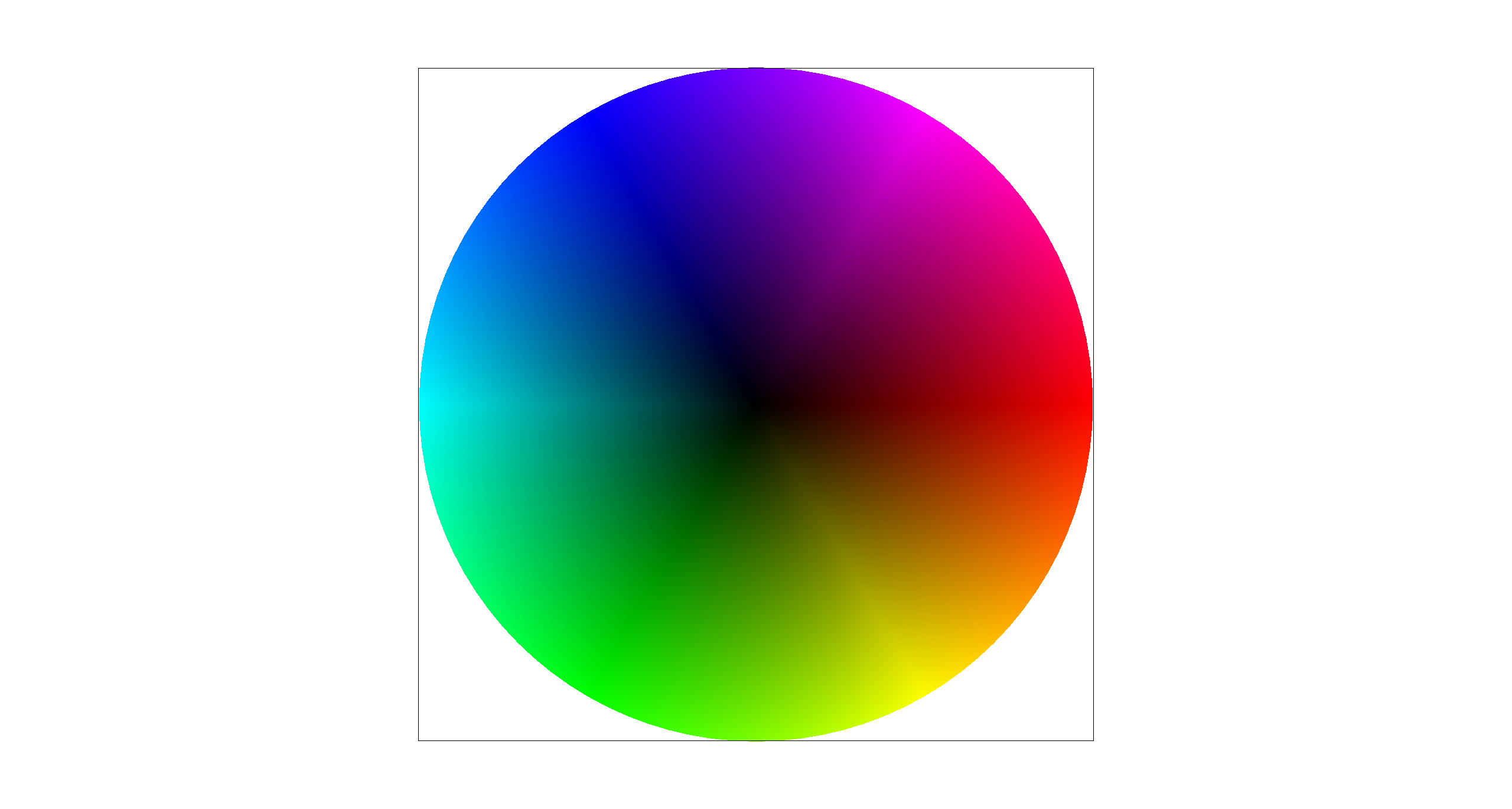
Task 4: Barycentric coordinates
Barycentric coordinates define a way to express a point with respect to the vertices of some triangle. In a sense, we can map from (x,y) in cartesian to some \(\alpha, \beta\) in barycentric. The useful part is that \(\alpha\) and \(\beta\) defines a third "coordinate" \(\gamma\) by \(\alpha + \beta + \gamma = 1\). These three coordinates represent weights on the vertices. To explain further, let's use an example.
|
|
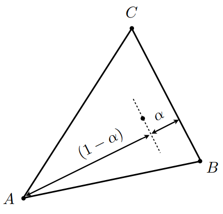
In the left figure above, we have a triangle with vertices A (Red), B (Blue), and C (Green). In barycentric coordinates, a point (x,y) inside the triangle would be \[(x,y) = \alpha A + \beta B + \gamma C\] We can think of each weight, let's first only consider \(\alpha\), as an interpolation between vertex A and the line BC. We draw a line from A perpendicular to BC and measure interpolation along it using \(\alpha \in [0, 1]\) (see figure on the right). The same idea applies to the other 2 weights.
The way these weights are restricted allows us to quite easily check if point P is inside of the triangle created by A, B, C. Once we have P in barycentric coordinates (\(\alpha, \beta\)), clearly both must be non-negative (or else we are already out of the triangle), and we can place the last restriction on \(\gamma\) implicitly by requiring \(\alpha + \beta <= 1\).
Since the weights basically parameterize interpolation, it lends quite nice to color interpolation (figure left). That is done
simply by implementing the equation above, but with Colors instead of vertices.
pair<float, float> weights = getBaryWeights(r, v0, v1, v2);
float alpha = weights.first;
float beta = weights.second;
if (alpha >= 0 && beta >= 0 && alpha + beta <= 1) {
	float gamma = 1 - weights.first - weights.second;
	// interpolated color is weighted sum
	Color color = weights.first * c0 + weights.second * c1 + gamma * c2;
	int buffer_pos = startPos + (j * width * dp) + i;
	sample_buffer[buffer_pos] = color;
}
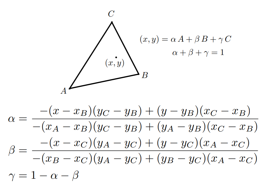
How Do You Get the Coordinates?
|
|
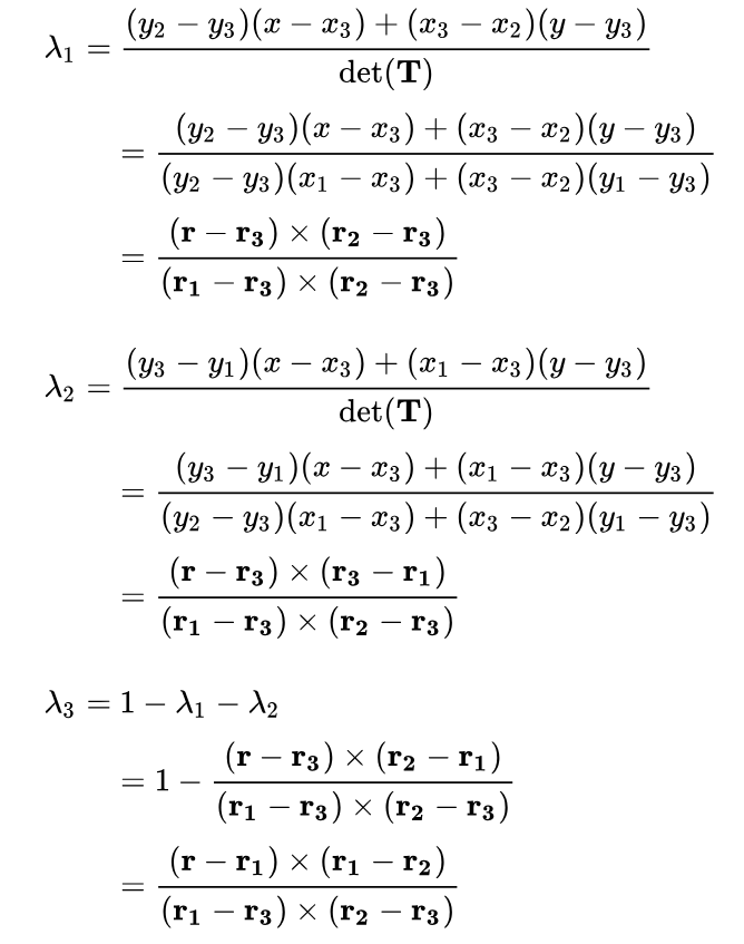
Barycentric coordinates can be easily calculated by cross products, so to simplify the code we will use the method in the right figure. First we vectorize our vertices and point.
// vectorize the sample point + vertices
Vector2D r(x + offset + i * dx, y + offset + j * dx);
Vector2D v0(x0, y0);
Vector2D v1(x1, y1);
Vector2D v2(x2, y2);
Then simply plug them into the equations:
pair<float, float> getBaryWeights(const Vector2D& r,
	const Vector2D& v0,
	const Vector2D& v1,
	const Vector2D& v2) {

	// formulas for alpha, beta can be represented neater as cross products
	float alpha = cross((r - v2), (v1 - v2)) / cross((v0 - v2), (v1 - v2));
	float beta = cross((r - v2), (v2 - v0)) / cross((v0 - v2), (v1 - v2));

	return pair<float, float>(alpha, beta);
}
Can you show a png screenshot of basic/test7.svg with the default viewing parameters and sample
rate 1?
Task 5: "Pixel sampling" for texture mapping
Our Texture Mapping Algorithm
1. Convert to uv Coordinates
We want to define a map between coordinates in the scene (our 2D cartesian plane) to coordinates on some texture. It is a convention to use uv coordinates, where \((u,v) \in [0,1]^2\). This mapping will allow us to take some coordinate (x,y) and apply a color to it that corresponds to its (u,v) location on the texture.
Luckily for us, the uv coordinates were given as parameters to rasterize_textured_triangle() so the only thing we need to worry about
is barycentric coordinates-- which we already have support for from Task 4!
Vector2D uv = weights.first * Vector2D(u0, v0) + weights.second * Vector2D(u1, v1) + gamma * Vector2D(u2, v2);
Color color;
// decide which sampling to use
if (psm == P_NEAREST) {
    color = tex.sample_nearest(uv);
}
else if (psm == P_LINEAR) {
    color = tex.sample_bilinear(uv);
}
sample_buffer[startPos + (j * width * dp) + i] = color;
The barycentric coordinate weights can be used directly on the uv vertices to get (x,y) in uv coordinates, which is then passed to our sample functions.
2. Sample
We can either sample nearest or sample bilinearly. Firstly, we need to scale (u,v) to the size of the texture.
float u = uv[0] * (mip.width - 1);
float v = uv[1] * (mip.height - 1);
(Note: a very silly mistake I made was not subtracting 1 from the dimensions and getting segmentation faults!)
For nearest sampling, just round these values and index the map.
return mip.get_texel(round(uv[0] * (mip.width - 1)), round(uv[1] * (mip.height - 1)));
For bilinear it's a little more complicated. We grab the four closest texels,
// coords of top-left texel
int x = floor(u);
int y = floor(v);

// interpolation weights
float s = u - x;
float t = v - y;

// top left texel
Color c00 = mip.get_texel(x, y);
// top right texel
Color c01 = mip.get_texel(x + 1, y);
// bottom left texel
Color c10 = mip.get_texel(x, y + 1);
// bottom right texel
Color c11 = mip.get_texel(x + 1, y + 1);
Then interpolate across the top and bottom rows, and once more between those two results (do we really have to call it lerping??):
// bilinear interpolation btwn top (c0) and bottom (c1) rows
Color c0 = c00 * (1 - s) + c10 * s;
Color c1 = c01 * (1 - s) + c11 * s;

// bilinear interpolation btwn both results
return c0 * (1 - t) + c1 * t;
What's the difference between nearest-pixel and bilinear sampling?
- In sample_nearest, we take the uv coordinates in [0, 1] and scale them to the texture's resolution based on the current mipmap level by multiplying the coordinates by the mip width or height subtracting 1. We then use the round function to find the nearest texel to those coordinates.
- In sample_bilinear, similar logic is applied to scale the uvs to the texture space but we don't only pick one texel. After computing the four surrounding texels c00, c01, c10, and c11, we interpolate their values. Then the interpolation weights are computed based on a fraction of the uv coordinates given.
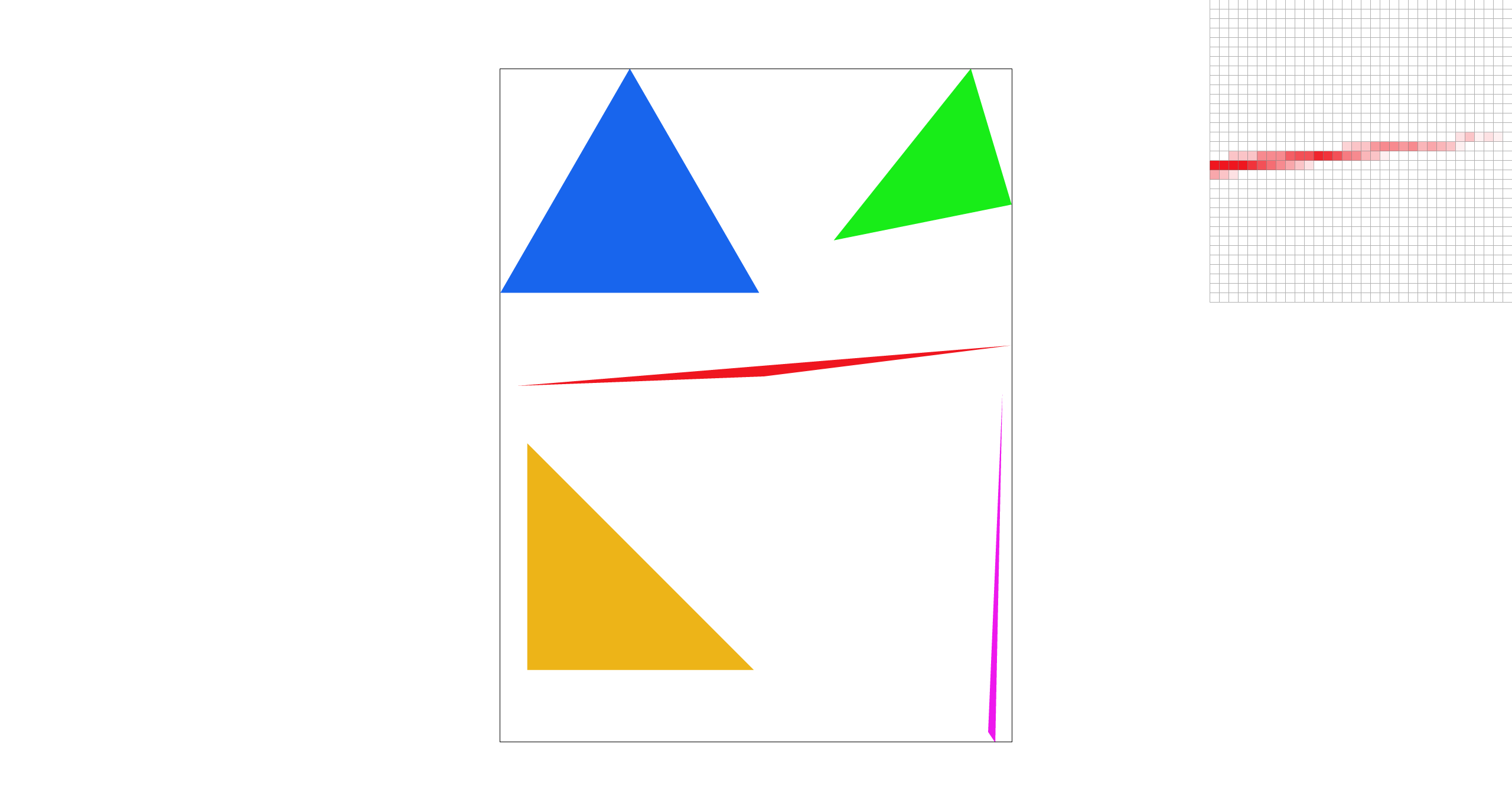
Comparison
|

|

|

|
In the top row, nearest-pixel sampling leaves some patches of missing gridline, which is visible when using bilinear sampling. However, bilinear seems to put a blur on everything which can lead to it looking worse in some situations. In the case of 16 samples per pixel, the difference is less noticeable because are getting better antialiasing from the supersampling. There will be a larger difference between the two methods in areas of an image that are higher frequency; the nearest-sample may also show a high-frequency output, but bilinear will blur it.
That's cool and everything, but what if we wanted to take things to another...level?
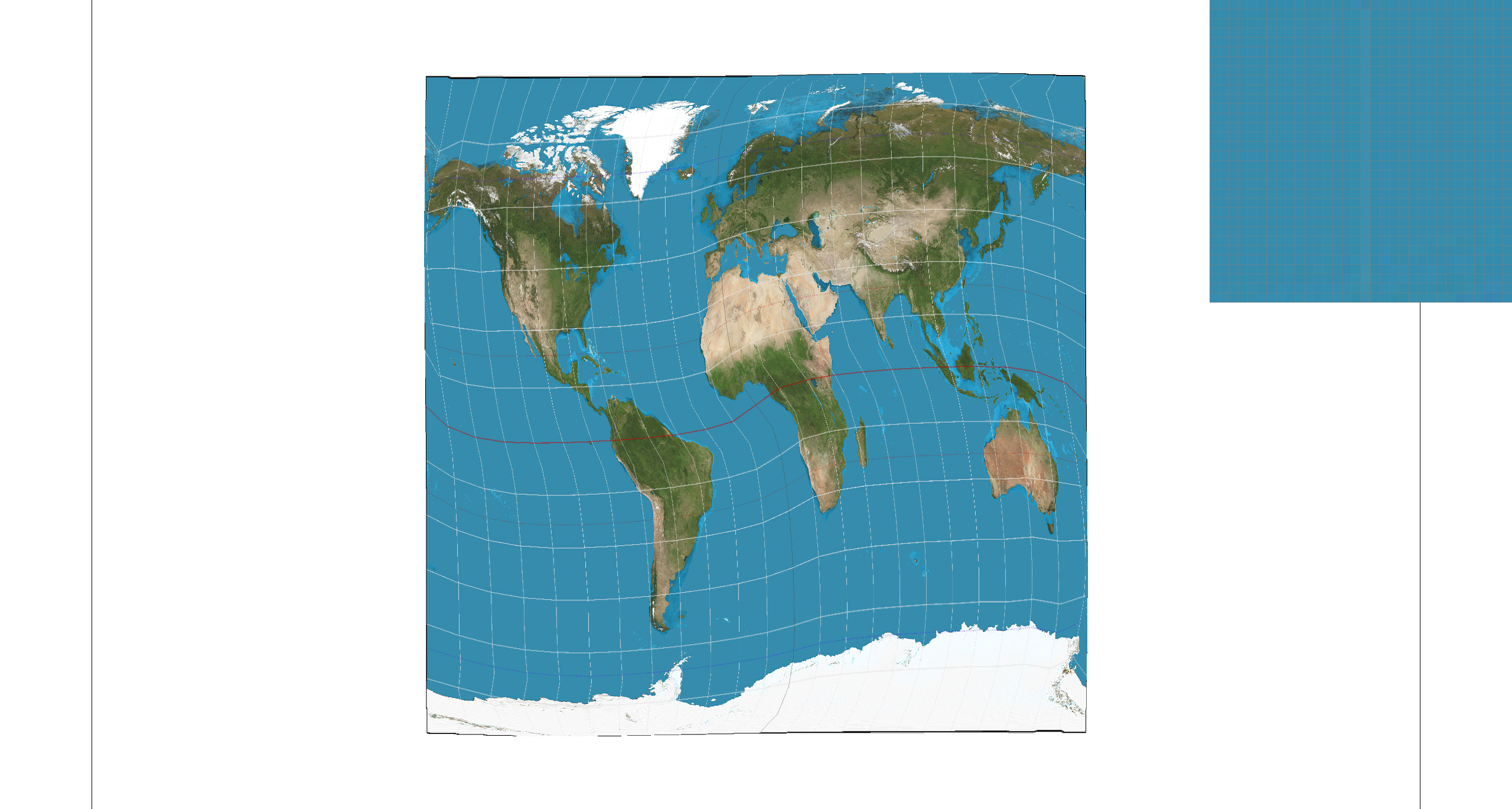
Task 6: "Level Sampling" with mipmaps for texture mapping
Sometimes when mapping textures onto curved surfaces, far away objects, or with perspective, the sampling methods we have implemented thus far may not cut it. For example, on a far away object, we may be trying to sample hundreds of pixels from the uv map onto only tens of pixels on the screen. Not only can this be inefficient, but it can also leave artifacts with higher frequency textures.
Enter the mipmap, a method of storing multiple copies of a texture at lower resolutions (called levels) in order to solve some of these problems.
Our Level Sampling Algorithm
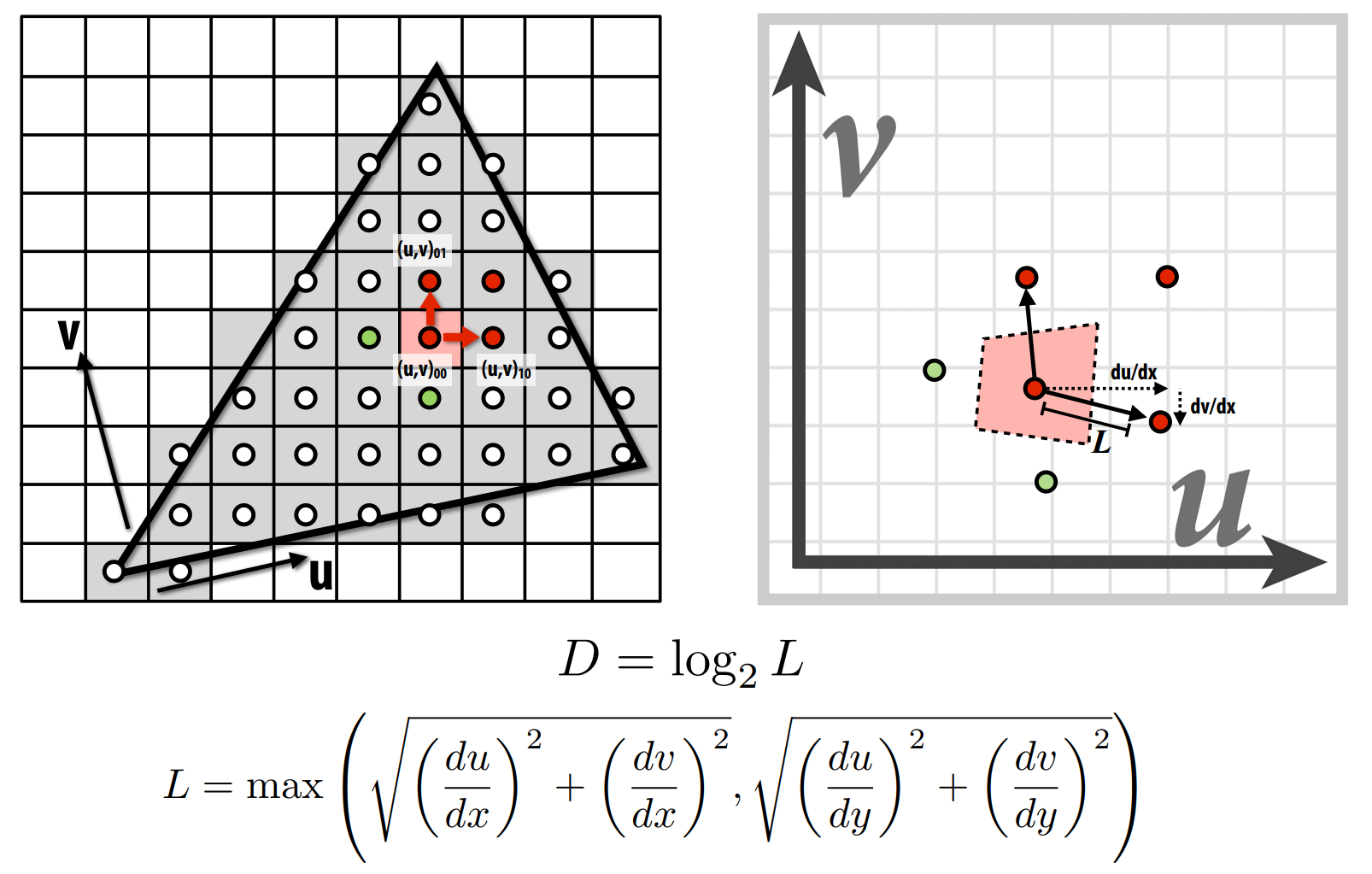
1. Fill SampleParams
First thing we want to know is what level of clarity we need from this texture in order for it to still look good. To do this, we need to calculate the correct mipmap level, which is given by some mathematical formulas (shown below). At its core, we are comparing how a differential (or in the discrete sense, single pixel) move in screen space corresponds to a move in uv space. For example, in the x-direction this is represented by \(\frac{du}{dx}, \frac{dv}{dx}\).
In the code we were gifted the SampleParams struct, which holds all the distance data we need to calculate
mipmap levels. Thus, in RasterizerImp::rasterize_textured_triangle() we just fill it with the needed data.
SampleParams uv;
uv.psm = this->psm;
uv.lsm = this->lsm;
uv.p_uv = weights.first * Vector2D(u0, v0) + weights.second * Vector2D(u1, v1) + gamma * Vector2D(u2, v2);
pair<float, float> dx_weights = getBaryWeights(r + Vector2D(dx, 0), r0, r1, r2);
pair<float, float> dy_weights = getBaryWeights(r + Vector2D(0, dx), r0, r1, r2);
gamma = 1 - dx_weights.first - dx_weights.second;
uv.p_dx_uv = dx_weights.first * Vector2D(u0, v0) + dx_weights.second * Vector2D(u1, v1) + gamma * Vector2D(u2, v2);
gamma = 1 - dy_weights.first - dy_weights.second;
uv.p_dy_uv = dy_weights.first * Vector2D(u0, v0) + dy_weights.second * Vector2D(u1, v1) + gamma * Vector2D(u2, v2);
Color color = tex.sample(uv);
Where our differential length is not a single pixel, but length of variable dx since we're working in conjunction
with supersampling. In the last line, we send all of this measurement data to the texture, where we will go next.
2. Calculate the Mipmap Level
We just use the formula from step 1 to calculate the level D, which is returned from Texture::get_level().
float Texture::get_level(const SampleParams& sp) {
	Vector2D diff_dx = sp.p_dx_uv - sp.p_uv;
	Vector2D diff_dy = sp.p_dy_uv - sp.p_uv;

	Vector2D duv_dx(diff_dx[0] * (width - 1), diff_dx[1] * (height - 1));
	Vector2D duv_dy(diff_dy[0] * (width - 1), diff_dy[1] * (height - 1));

	float du_dx = duv_dx[0];
	float dv_dx = duv_dx[1];
	float du_dy = duv_dy[0];
	float dv_dy = duv_dy[1];

	float L = max(sqrt(pow(du_dx, 2) + pow(dv_dx, 2)), sqrt(pow(du_dy, 2) + pow(dv_dy, 2)));
	return log2(L);
}
3. Handle Chosen Sampling Options
Now we just need to make some changes to Texture::sample() to handle the level sampling settings.
Firstly, we want to round D if we're using nearest level.
float D = 0;
if (sp.lsm != L_ZERO) {
    D = get_level(sp);
    if (sp.lsm == L_NEAREST) {
        D = round(D);
    }
    // somehow D can be negative/bigger than the mipmap size
    // so just account for that here
    if (D >= mipmap.size()) {
        D = mipmap.size() - 1;
    }
    else if (D < 0) {
        D = 0;
    }
}
Note that we also check that D is within our bounds; this fixes a bug where zooming too far in or out would cause problems.
Now we just make some additional changes to our sampling calls, using nested if loops to handle level sampling options.
Color color;
// decide which sampling to use
if (sp.psm == P_NEAREST) {
    color = sample_nearest(sp.p_uv, D);
    if (sp.lsm == L_LINEAR && D < mipmap.size() - 1) {
        float weight = D - floor(D);
        color *= 1 - weight;
        color += sample_nearest(sp.p_uv, D + 1) * weight;
    }

}
else if (sp.psm == P_LINEAR) {
    color = sample_bilinear(sp.p_uv, D);
    if (sp.lsm == L_LINEAR && D < mipmap.size() - 1) {
        float weight = D - floor(D);
        color *= 1 - weight;
        color += sample_bilinear(sp.p_uv, D + 1) * weight;
    }

}

return color;
Since the sample_nearest/bilinear functions floor D to an int anyways, we can call them on D for all types of lsm and simply compute an additional linear interpolation if we're using bilinear (the code inside of the nested if).
Different Sampling Techniques
From what we have discussed so far, we can compare our implemented sampling techniques on the basis of speed, memory usage, and antialiasing power.
- The simplest observation is that supersampling is slow and memory-heavy. Each time we increase the sample rate, we're scaling the size of the buffer. Every time we check a pixel we need to check all the subsamples, even if they end up all being the same color/not in the triangle. Despite this, it delivers a very accurate antialiasing technique, since we are basically rendering at a higher resolution and bringing it back down.
- Then we have pixel sampling, which conceptually seems the simplest, and would therefore seem to be the fastest. At its simplest is nearest pixel sampling: we only need to look at one pixel in the uv texture map, so lookup is quick, but as a result, it is not great at antialiasing high frequency areas. Bilinear pixel sampling is a little smoother, but can still struggle at high frequencies or with something like depth.
- Then there is level sampling, somewhere in between the two previously mentioned techniques, as it is more involved than pixel sampling but not as exhaustive as supersampling. A mipmap may take up more space, but at only 4/3 the size of the originally image it is not much more spacially inefficient. Level sampling can deal with aliasing caused by depth issues, known as texture minification. The use of trilinear filtering is great at antialiasing, but is slower than bilinear filtering due to a second mipmap lookup.
Comparisons

|
|
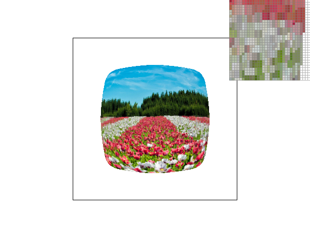
|
|
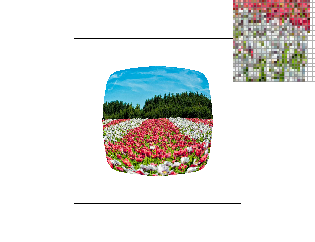
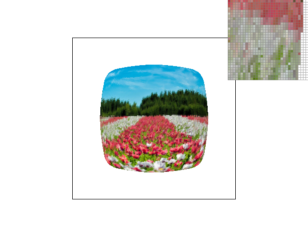
Failed Attempts at Examples
I tried really hard to find a funny photo that could show off the sampling implementations but none of them were high enough frequency. I'm still going to put them here though because I like them.
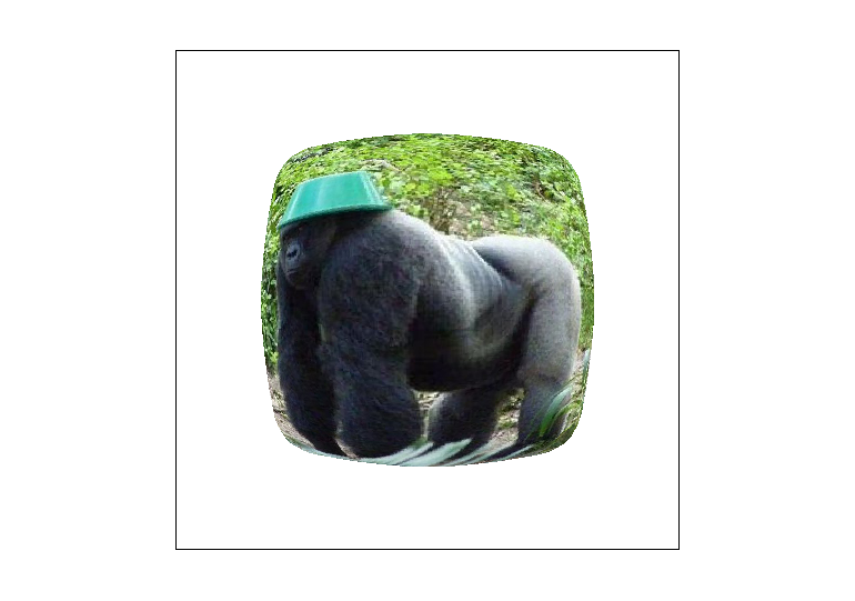
|
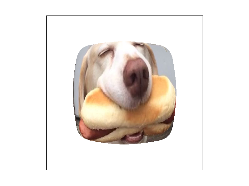
|
|
|