CS184 Summer 2025 Homework 3 Write-Up
Link to webpage: https://cs184.snoopboopsnoop.com/hw3
GitHub Repository (Private): https://github.com/cal-cs184/hw-pathtracer-updated-jcheng3
Also, none of the MathJax inline math loaded in, so check out the website for that too. I've marked all places with MathJax with an asterisk.*
Overview
In Homework 3, we built a path tracer from its ray generation, to its bounding volume hierarchy structure, to its direct illumination, to its global illumination, to its adaptive sampling. In part 1, we implemented camera ray generation based on the screen coordinates normalized, used random pixel sampling wih anti-aliasing, and built functions for triangle and sphere intersections. Then in part 2, we built a recursive BVH structure to organize primitives and optimize ray-primitive intersection. Building upon this, we implemented zero-bounce radiance and direct lighting techniques using uniform hemisphere sampling and light sampling. To create soft shadows and realistic effects, we implemented BSDF-based ray sampling, multiple bounce path tracing, and Russian Roulette. Lastly, we added adaptive sampling to decide when to stop sampling per pixel.
I found doing part 3 the most interesting, especially testing the comparisons between uniform hemisphere sampling and light sampling. Seeing the noise reduction on the light sampling was very insightful to see the effects that sampling toward light sources have. Sampling in directions more likely to add light makes each sample more meaningful since less samples are needed in total to get a well-lit image. Making small changes to result in a big visual difference feels very clever to me, and I like how the simulated scene ends up looking more realistic than the uniform hemisphere sampling. -Crystal
I've always heard about ray-tracing through the context of video game graphics and GPU hardware, and just vaguely knew that it involved "simulating" light rays in order to render. I also assumed it was some complicated industrial thing that I couldn't do from home, so it felt very rewarding and cool to be able to implement path tracing in this homework. I struggled the most implementing global illumination, but at the same time I enjoyed getting it to work the most. Additionally, I felt that I much better understood the concepts from lectures 11 - 13 by implementing them in this homework, especially for things like radiance and BSDFs. -Walter
Part 1: Ray Generation and Scene Intersection
Ray Generation and Primitive Intersection
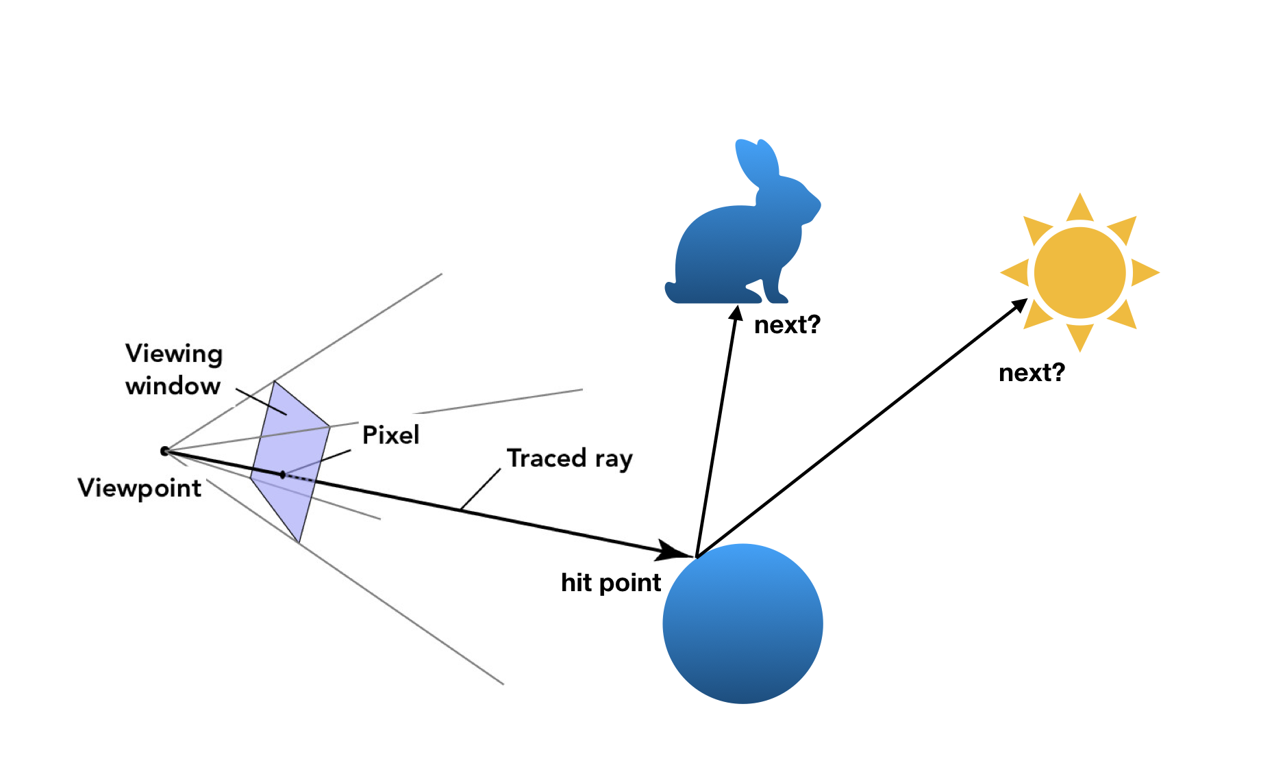
As noted in our textbook, Fundamentals of Computer Graphics by Peter Shirley and Steve Marschner, ray-tracing is an image-order algorithm implemented in order to render 3d scenes. This is because unlike the 2D rasterizer (HW 1), we now need to figure out what the camera will be looking at in order to color a pixel.
At its most basic, a ray-tracing algorithm is this: for each pixel, compute a "viewing ray". Find the first primitive that intersects this ray at some time t, and using the surface normal at this intersection point we can compute a pixel color.
So, it looks like we have to implement ray generation and primitive intersection, doesn't it?
Ray Generation
Our ray generation starts with the generate_ray function in camera.cpp.
This function translates an (x, y) coordinate from screen space to a ray in world space
pointing from the camera to the corresponding point on the virtual camera sensor.
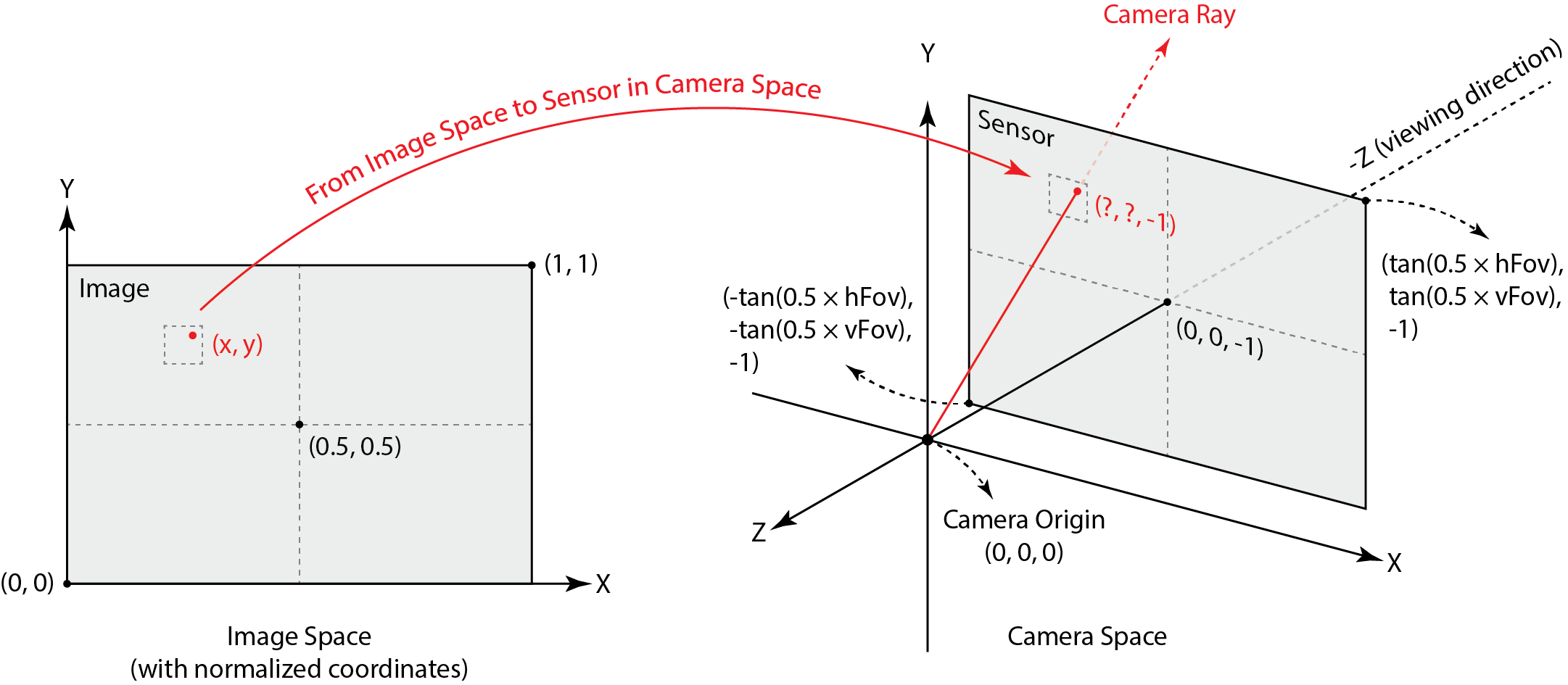
Thankfully the coordinates in image space are taken to be normalized, so we can just use linear interpolation to translate from image coordinates to sensor coordinates. From the diagram above, we see that the corner coordinates are mapped as so:* \[(0, 0) \to (-\tan\left(\frac{\text{hFov}}{2}\right), -\tan\left(\frac{\text{vFov}}{2}\right), -1)\] \[(1, 1) \to (\tan\left(\frac{\text{hFov}}{2}\right), \tan\left(\frac{\text{vFov}}{2}\right), -1)\]
We've done linear interpolation so many times. It's the same.
// get coordinates of bottom left and top right
float minX = -tan(0.5 * hFov * PI / 180.0);
float minY = -tan(0.5 * vFov * PI / 180.0);
float maxX = -minX;
float maxY = -minY;

// interpolate
float camX = (1 - x) * minX + x * maxX;
float camY = (1 - y) * minY + y * maxY;
Now to turn this coordinate into a Ray, we can just create the vector in camera space, normalize it, and then
rotate it to world space using the provided c2w matrix.
// get ray direction
Vector3D dir(camX, camY, -1);
dir.normalize();

Ray result = Ray(pos, c2w * dir);
result.min_t = nClip;
result.max_t = fClip;

return result;
Triangle Intersection
Given a Ray and a Triangle, we want to know if they intersect, and if they do,
at what time t (and also what the surface normal is, and some other stuff built into the Intersection
class). There are many methods for computing this, but we settled on the Möller-Trombore Algorithm.
Our implementation is based off the Wikipedia page for the algorithm. It seems redundant to explain the whole thing, but at its core, using barycentric coordinates (HW 1), we can express the equation of intersection as a system of equations/matrix equation:

Using Cramer's Rule (something I haven't touched since community college linear algebra) we can solve for t, u, and v.
For those unfamiliar, Cramer's Rule says that for a system*
\[A\vec{x} = \vec{b}\]
The values in x can be solved for by

Where* \(A_i\) is the matrix A with the ith column replaced with b.
// solve system using Cramer's Rule
Vector3D b = r.o - p1;
Matrix3x3 A;
A.column(0) = -r.d;
A.column(1) = v12;
A.column(2) = v13;

float det = A.det();

float result[3]; // [t, u, v]
for (int i = 0; i < 3; ++i) {
	Matrix3x3 Ai(A);
	Ai.column(i) = b;
	result[i] = Ai.det() / det;
}
Then, after checking our edge conditions for baycentric coordinates and our t range, we can claim intersection.
// verify barycentric coordinates and non-negative t
float t = result[0];
float u = result[1];
float v = result[2];
if (t >= r.min_t && t <= r.max_t && u >= 0 && v >= 0 && u + v <= 1) {
	if (isect != nullptr) {
		r.max_t = t;
		isect->t = t;
		isect->n = (1 - u - v) * n1 + u * n2 + v * n3;
		isect->primitive = this;
		isect->bsdf = bsdf;
	}
	return true;
}
return false;
Also note that when I explained ray-tracing above, it was at its simplest. In task 2, rather than generating one ray
per pixel, we implemented the raytrace_pixel function, which computes a uniform average of multiple rays
(randomly generated around the pixel) and displays that color.
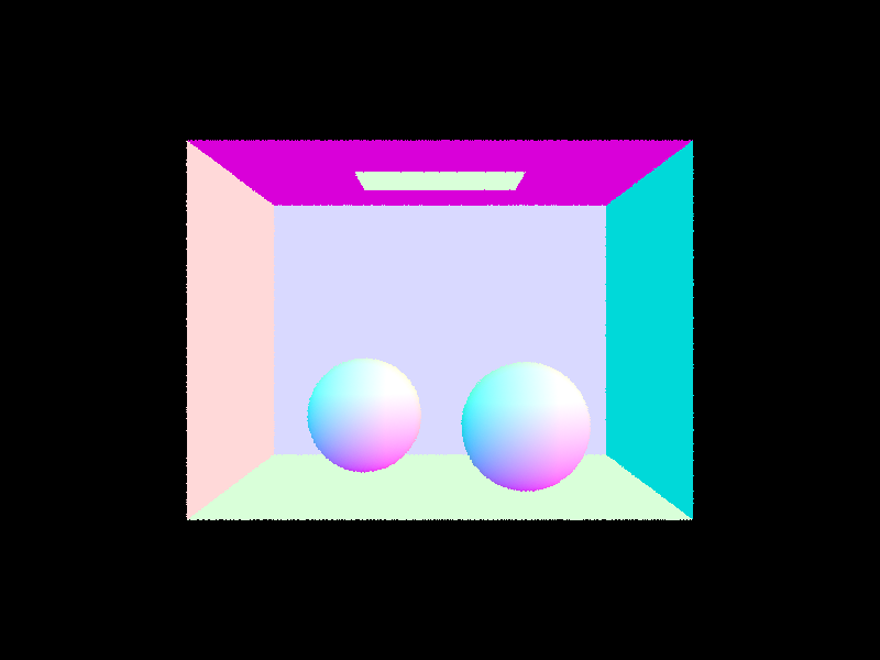
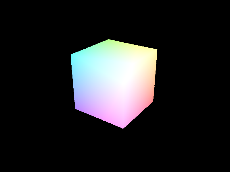
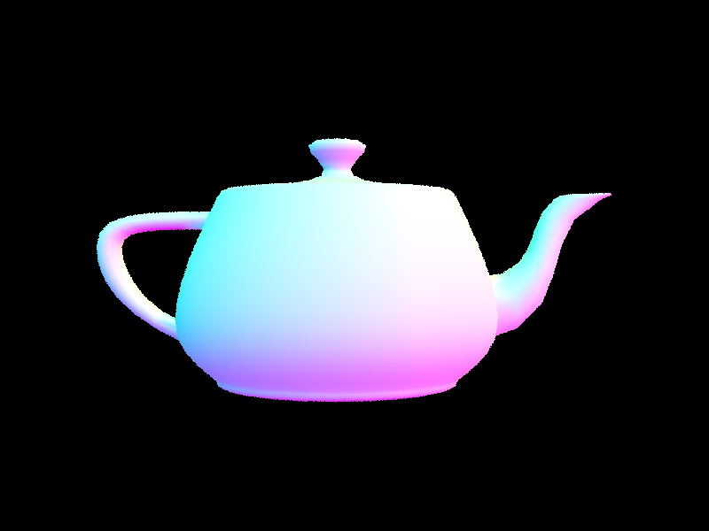
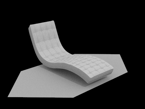
Some images
Part 2: Bounding Volume Hierarchy
Our Algorithm
The BVHAccel::construct_bvh algorithm essentially recursively creates a binary tree with the
base case of having less than the maximum allowed number of primitives within the node's bounding box.
Walkthrough
The starter code already does Node construction for us, so we just implemented the recursion. If
our node's bounding box has too many primitives, then split.
// get number of primitives in box, helps with iterator indexing
int num_prims = end - start;

// check if we need to split
if (num_prims > max_leaf_size) {
    ...
}
To maximize our benefit in a simple way, we will split along the longest axis on the current node's bounding box.
This is calculated and stored in max_index (0 = x, 1 = y, 2 = z). The heuristic to pick where on the axis
to split is the average max_index value across all of the primitives' centroids:
// get average centroid (average pt along all axes)
Vector3D average;
for (auto p = start; p != end; p++) {
    average += (*p)->get_bbox().centroid();
}
average /= num_prims;
Now that we have chosen an axis and a point along the axis to split, we have to construct new start, end iterators
for the left and right children of the current node. To save memory, we implicitly use only the BVHAccel member primitives
and rearrange it for our purposes. So, for the section of primitives that is inside of our current node, namely the elements
in [start, end), we will sort them based on their axis, and then assign left and right iterators.
// recursion and also some iterator logic that makes me want to kill myself
// sort this node's primitives by value on split axis
sort(start, end, [max_index](const Primitive* a, const Primitive* b) {
    return a->get_bbox().centroid()[max_index] < b->get_bbox().centroid()[max_index];
    });

// get iterators for the left/right split
auto rightBegin = find_if(start, end, [max_index, average](const Primitive* a) {
    return a->get_bbox().centroid()[max_index] > average[max_index];
    });
auto rightEnd = end;

// handles infinite recursion if we split and right side has nothing
// occurs when all primitives are in the same split axis (aka equal to average)
if (rightEnd == rightBegin || rightEnd - rightBegin == num_prims) {
    rightBegin = rightEnd - (num_prims / 2);
}

// use number of primitives to calculate left iterators
// i'm pretty sure sorting fucks up the start iterator so i don't want to use it
auto leftEnd = rightBegin;
auto leftBegin = leftEnd - (num_prims - (end - rightBegin));
An Edge Case
Notice that in the code above, we have an if statement between the right and left iterator assignments. This handles the case where
"the split point is chosen such that all primitives lie on only one side of the split point", a segfault noted in the implementation notes
in the homework spec. For our heuristic, this occurs when every primitive lies on the same point along the max_index axis, i.e.
rightBegin gets assigned to either the start of the section or the end, depending on floating point comparison. To remedy, we
just put half the primitives in left and half of them in right.
Now all we need to do is recurse.
// recurse
node->l = construct_bvh(leftBegin, leftEnd, max_leaf_size);
node->r = construct_bvh(rightBegin, rightEnd, max_leaf_size);
And in the case that we are below the max_leaf_size, set left and right to nullptr.
else { // leaf node
    node->start = start;
    node->end = end;
    node->l = nullptr;
    node->r = nullptr;
}
return node;
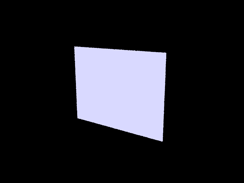
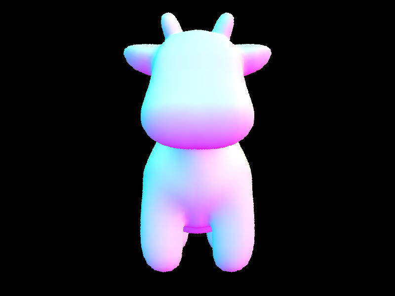
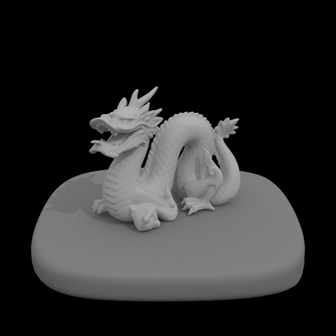
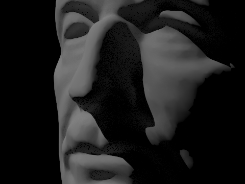
Some images rendered using BVH implementation - these would have taken forever without!
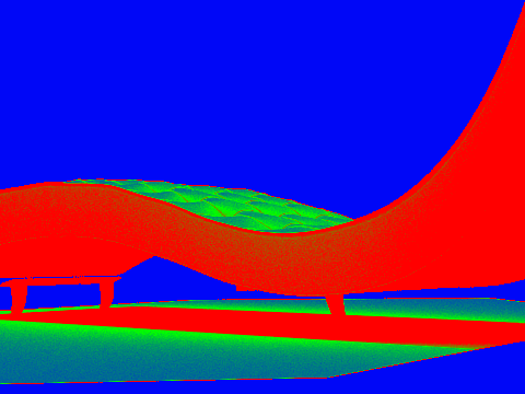
Comparing Render Times (No BVH vs. BVH Acceleration)


Comparing each of the image render times side-by-side, the rendering speedup caused by BVH acceleration is incredibly clear. Although scenes with simple meshes (the top row above) did not have very long rendering times to begin with, the efficiency becomes much more clear when the meshes get more complicated (bottom row). This is because the BVH structure allows us to descend a tree in order to check for ray intersection rather than check every single primitive in the mesh (you can see why more complicated meshes would take so long).
Part 3: Direct Illumination
In Part 3, we implement realistic shading by simulating light transport in the scene using pathtracer function
est_radiance_global illumination function as the main rendering loop. What allows this are the
BSDF (Bidirectional Scattering Distribution Function), adding zero-bounce illumination, implementing direct lighting estimations, and adding one-bounce radiance.
Diffuse BSDF
This function takes in both wo and wi and returns the evaluation of the BSDF for those two directions.
Vector3D DiffuseBSDF::f(const Vector3D wo, const Vector3D wi) {

    return reflectance / PI;

}
The sample_f function evaluates diffuse lambertian BSDF. This function takes in only wo and provides pointers for wi and pdf,
which is then assigned by this function. After sampling a value for wi, it returns the evaluation of the BSDF
at (wo, *wi).
Vector3D DiffuseBSDF::sample_f(const Vector3D wo, Vector3D *wi, double *pdf) {

     *wi = sampler.get_sample(pdf);

     return f(wo, *wi);
}
Zero-Bounce Illumination
To add zero-bounce illumination, we return the light that results from no bounces of light using
the get_emission() function.
Vector3D PathTracer::zero_bounce_radiance(const Ray &r, const Intersection &isect) {

  return isect.bsdf->get_emission();

}
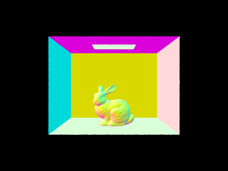
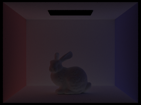
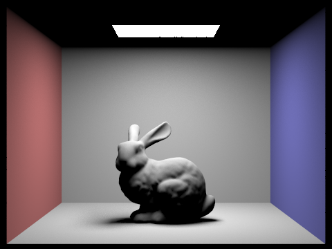
This results in an all black image, with only the window of light being emitted from the ceiling. We are unable to view the bunny with zero-bounce illumination.
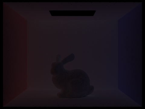
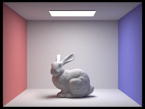
Direct Lighting by Uniform Hemisphere Sampling
We are given the following estimate_direct_lighting_hemisphere function as a base.
We estimate the lighting from this intersection coming directly from a light, sampling uniformly in a hemisphere.
 Vector3D PathTracer::estimate_direct_lighting_hemisphere(const Ray &r, const Intersection &isect) {
  // make a coordinate system for a hit point
  // with N aligned with the Z direction.
  Matrix3x3 o2w;
  make_coord_space(o2w, isect.n);
  Matrix3x3 w2o = o2w.T();

  // w_out points towards the source of the ray (e.g.,
  // toward the camera if this is a primary ray)
  const Vector3D hit_p = r.o + r.d * isect.t;
  const Vector3D w_out = w2o * (-r.d);

  // This is the same number of total samples as
  // estimate_direct_lighting_importance (outside of delta lights). We keep the
  // same number of samples for clarity of comparison.
  int num_samples = scene->lights.size() * ns_area_light;

  Vector3D L_out(0, 0, 0);

}
For Part 3, we add Monte Carlo Integration. We also update est_radiance_global_illumination to return direct lighting instead of normal shading.
L_out = zero_bounce_radiance(r, isect);
To implement Monte Carlo, we first sample uniformly on hemisphere, then create ray from hit point in sampled direction.
If the ray hits a light source, we get emission from the intersected object. Then if we hit something
emissive, we continue with evaluating the BSDF. Normally the cos(theta) is a dot product, but because
the normal is simply (0, 0, 1), we can set it to wi_local.z.
  for (int i = 0; i < num_samples; i++) {
    // sample uniformly on  hemisphere
    Vector3D wi_local = hemisphereSampler->get_sample();

    // convert to world space
    Vector3D wi_world = o2w * wi_local;

    // create ray from hit point in sampled direction
    Ray sample_ray(hit_p, wi_world);
    // no self-intersection
    sample_ray.min_t = EPS_F;

    // if ray hits a light source
    Intersection light_isect;
    if (bvh->intersect(sample_ray, &light_isect)) {
      // get emission from the intersected object
      Vector3D emission = light_isect.bsdf->get_emission();

      // continue if we hit something emissive
      if (emission.illum() > 0) {
        // evaluate BSDF
        Vector3D f = isect.bsdf->f(w_out, wi_local);

        // dot prod but normal is just (0, 0, 1)
        double cos_theta = wi_local.z;

        // add if cos_theta above horizon
        if (cos_theta > 0) {
          // for uniform hemisphere sampling
          double pdf = 1.0 / (2.0 * PI);

          // monte carlo estimate
          L_out += emission * f * cos_theta / pdf;
        }
      }
    }
  }

  // avg all samples
  return L_out / num_samples;
If the cos(theta) is greater than 0, that means it is above the horizon and we use the
equation pdf = 1/2pi for uniform hemisphere sampling. The Monte Carlo estimate is then just the current L_out
adding emission * f * cos_theta / pdf. Lastly, we return the average of all samples, which we obtain by dividing the total
number of samples.
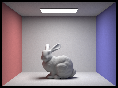
Importance Sampling
The problem with uniform hemisphere sampling is that we're wasting a lot of rays. Most of them don't intersect with light. Imagine trying to get a ray to hit a point light, the probability is basically 0. So, we can turn to a more efficient method of sampling: light sampling, where instead of randomly choosing where to sample, we will sample each light.
The algorithm is very similar to uniform sampling, so much of the syntax is very similar.
We're implementing importance sampling in PathTracer::estimate_direct_lighting_importance
To start, we will loop over all lights in the scene.
// sample from all lights in scene
vector<SceneLight*> lights = scene->lights;
int num_samples = lights.size();

for (SceneLight* light : lights) {
    int light_samples = ns_area_light;
    ...
}
In the case that we have a point light, we will only sample one time, since the samples will all be the same.
// sample from point lights only once
if (light->is_delta_light()) {
    light_samples = 1;
}
Now we just sample the light light_samples times.
Vector3D wi; // omega in (world coordinates)
double dist; // distance between hit_p and light
double pdf; //
Vector3D emission = light->sample_L(hit_p, &wi, &dist, &pdf);
Vector3D wi_local = w2o * wi;

if (wi_local.z < 0) continue;
Checking for Shadows
When we sample a light, we need to know whether or not the light actually hits our point.
So we send a ray out in the sample direction we received, wi. If we don't
intersect anything, and therefore do get light from the source, we will calculate its
radiance and add it to our Monte Carlo estimator.
Ray sample_ray(hit_p, wi);
sample_ray.min_t = EPS_F;
sample_ray.max_t = (dist - EPS_F);

Intersection light_isect;
if (!bvh->intersect(sample_ray, &light_isect)) {
    // evaluate BSDF
    Vector3D f = isect.bsdf->f(w_out, wi_local);

    // dot prod but normal is just (0, 0, 1)
    double cos_theta = wi_local.z;

    // add if cos_theta above horizon
    if (cos_theta > 0) {
        // monte carlo estimate
        currLight += emission * f * cos_theta / pdf;
    }
}
Note the use of EPS_F to make sure we don't accidentally intersect with either
our current primitive or the light. (we know we'll intersect with the light eventually!)
Then, like for uniform sampling, we just normalize by our samples.
for (int i = 0; i < light_samples; i++) {
    ...
    L_out += currLight / light_samples;
}
return L_out / num_samples;
Show some images rendered with both implementations of the direct lighting function.
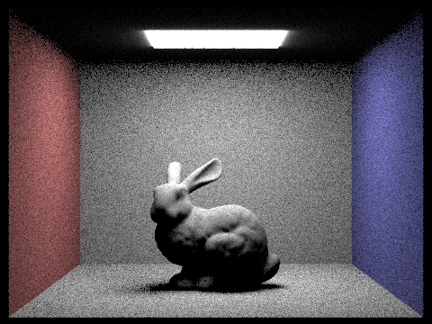


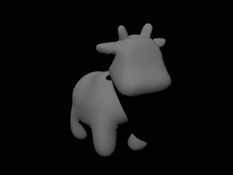
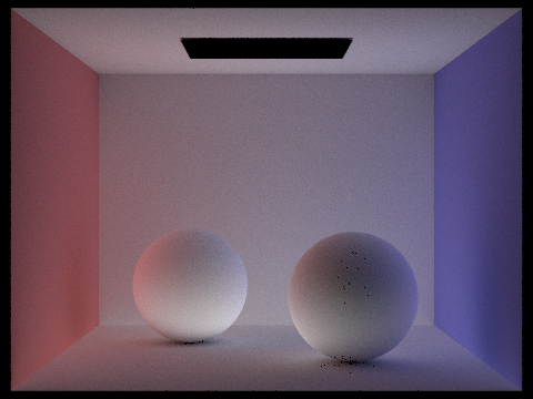
Since cow.dae only has a point light, when we use uniform hemisphere sampling, the probability that the ray intersects with light is near 0 because of floating point comparison. Thus the cow renders as a black image. Light sampling fixes this problem, which is why we are able to view the cow.
Focus on one particular scene with at least one area light and compare the noise levels in soft shadows when rendering with 1, 4, 16, and 64 light rays (the -l flag) and with 1 sample per pixel (the -s flag) using light sampling, not uniform hemisphere sampling.
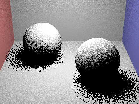
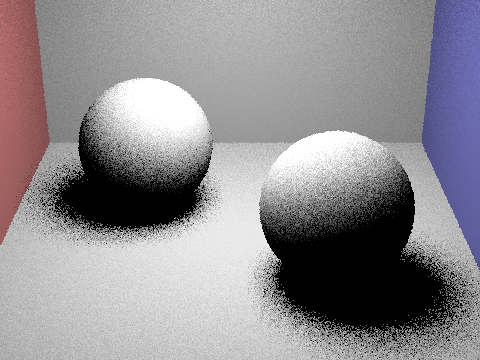

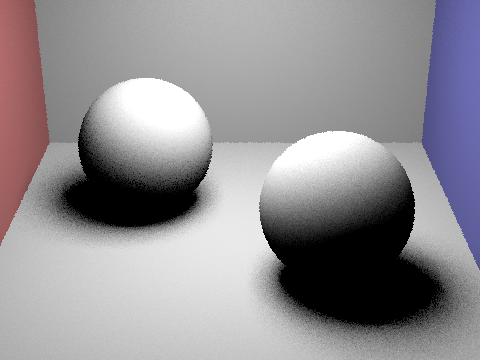
The more light rays used in light sampling, the less noise we see and a clearer image is rendered. Observing the soft shadows under the spheres, we see the noise levels are much higher, resulting in a grainy image.
Compare the results between uniform hemisphere sampling and lighting sampling in a one-paragraph analysis.
Uniform hemisphere sampling is best for when there are many evenly distributed light sources while light sampling is best for scenes with varying light source sizes. As seen from the images above, scenes with uniform hemisphere sampling has heavy noise since rays are randomly chosen from all directions of the hemisphere. On the other hand, light sampling has rays sampled from the direction that the light sources are located at and helps illuminate scenes more accurately using fewer samples. So although light sampling is more complex to implement, it performs better than uniform hemisphere sampling in noise and lighting.
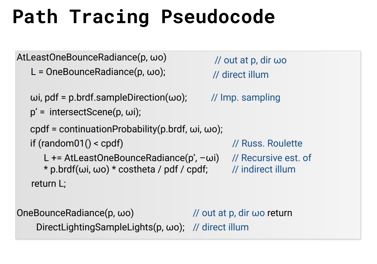
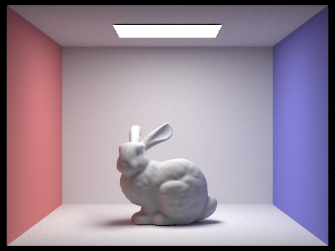
Part 4: Global Illumination
Our Implementation
|
|
The direct illumination that we implemented in Part 3 doesn't tell the whole story. What we see so far in our render is only all of the light that is emitted from a source, bounces off an object, and goes to the camera sensor (single-bounce). What about all of the other light? In reality, light may bounce around a large number of times before hitting our eyes, so we aim to replicate this "indirect" illumination by implementing global illumination.
Walkthrough
In our implementation we have a maximum number of bounces, which is passed in as a command line argument,
and in part 3 we also have a Russian Roulette factor to continuing a ray path, given by a termination
probability termination_prob.
We'll start with the simplest function we edited, est_radiance_global_illumination.
We still want zero-bounce illumination, but also all other bounces:
L_out = zero_bounce_radiance(r, isect);
if (max_ray_depth > 0) {
    Vector3D more_bounce = at_least_one_bounce_radiance(r, isect);
    if (isAccumBounces) {
        L_out += more_bounce;
    }
    else {
        L_out = more_bounce;
    }
}
Notice the variable isAccumBounces. There are if-else statements scattered around to handle
whether or not our path tracing is cumulative, but I will not go on to point them out.
Our actual algorithm is contained within at_least_one_bounce_radiance, where we implemented
the pseudocode shown at the header of this section. Firstly, we want to do one bounce direct lighting at
our intersection point of interest.
L_out = one_bounce_radiance(r, isect);
// check if we've hit depth
if (r.depth == max_ray_depth) {
    return L_out;
}
Keeping track of ray depth
As a small aside, we keep track of ray depth through the Ray.depth member variable. In our pathtracer
we initialize every ray with depth = 1:
Ray ray = camera->generate_ray(x_sample, y_sample);
ray.depth = 1;
We start at 1 because all depth 0 rays are handled in zero_bounce_radiance. Then, for each
bounce ray recursively defined in at_least_one_bounce_radiance, we increment its depth.
if (!coin_flip(termination_prob)) {
    // sample bsdf to get a direction to continue
    ...

    Ray sample_ray(hit_p, wi_world);
    sample_ray.min_t = EPS_F;
    sample_ray.depth = r.depth + 1; // new ray is 1 more deep

    // get intersection with the next surface along ray
    ...
}
Also notice that we check whether or not to continue using the coin_flip() function from
random_util.h
Keep on keeping on...
Now we want to pick a direction to bounce; this is handled by sampling the bsdf of the primitive we've hit.
Vector3D reflectance = isect.bsdf->sample_f(w_out, &wi_local, &pdf);
Then see if we intersect anything along that ray direction.
// get intersection with the next surface along ray
Intersection next_isect;
if (bvh->intersect(sample_ray, &next_isect)) {
    Vector3D next_light;

    Vector3D emission = next_isect.bsdf->get_emission();
    Vector3D bounceRadiance;
    // check if next intersection is a light, if not then recurse
    ...
}
If we do intersect something, we'll recurse through at_least_one_bounce_radiance to
get the radiance from the next bounce in our w_in direction. Taking this radiance,
we calculate the radiance at our original bounce location from the "next" bounce using the
reflection equation. Since we're only sampling once, the calculation is simple. We also make sure to
normalize by the continuation probability.
// check if next intersection is a light, if not then recurse
if (emission.illum() == 0) {
    bounceRadiance = at_least_one_bounce_radiance(sample_ray, next_isect);
    double cos_theta = wi_local.z;
    if (cos_theta > 0) {
        next_light = bounceRadiance * reflectance * cos_theta / pdf / (1-termination_prob);
    }
}
Lastly, we just return the radiance calculated (or sum it with L_out if we
are accumulating).
if (isAccumBounces) {
    L_out += next_light;
}
else {
    return next_light;
}
Some Global Illumination Images

Direct vs. Indirect Lighting Comparison
(The images were rendered at 1024 samples per pixel, 4 ray samples per light, and maximum depth 100 with Russian Roulette factor 0.35)
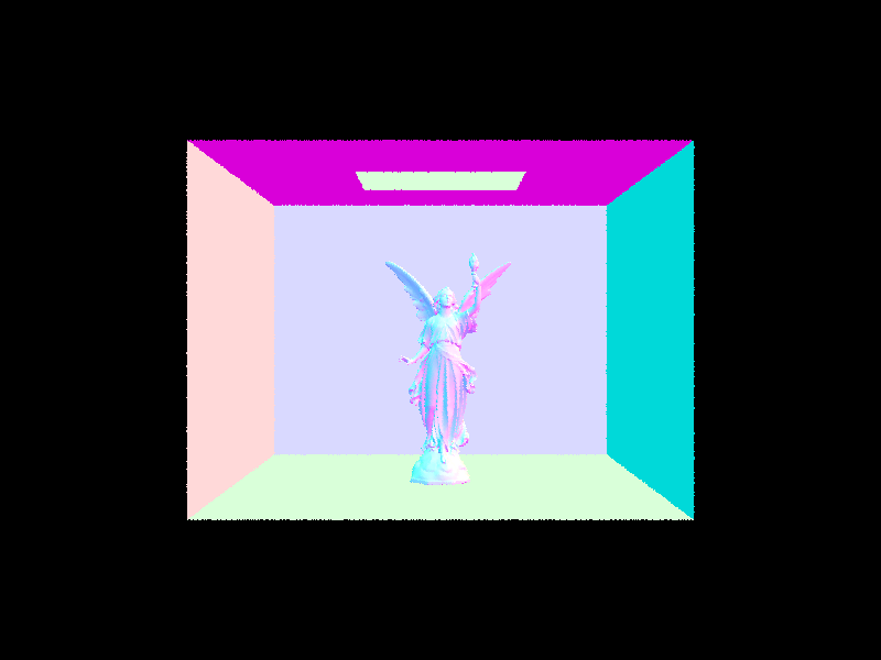
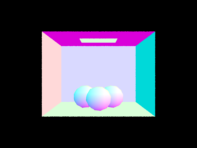
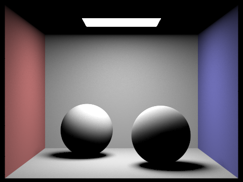
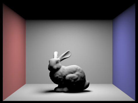
The direct lighting render makes sense; it's all light shining from the light at the top directly onto the scene. The balls are lit from the top, and the walls and floor are lit. Notice that the roof is completely dark! This makes sense, since no light can shine on the roof if the light is coming from the roof.
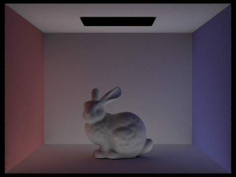
The indirect lighting tells the rest of the story. The area light at the top is dark. This is because we stop pathtracing when we hit the light (since we're basically backtracking, and the light is the source). In reality, light may bounce back off of the light since it is a physical object, but it's (probably) negligible. Note, also, that we have color bleeding! Light is reflecting off the walls and onto the balls. Lastly, the balls are lit from below, caused by light reflecting off the floor and onto to the balls.
Try Pulling This One Out of a Hat!

(The images were rendered at 1024 samples per pixel, 4 ray samples per light, and Russian Roulette factor 1.0)
Like mentioned above, bounce 2 helps our image by rendering all the light that bounces off the ground and back up at the bunny, as well as all the light that bounces off the walls and onto the bunny. This creates the underlighting and color bleeding we see. Whereas in the previous bounces only certain areas are lit up (e.g. the roof, the floor), in bounce 3 we get a more dim but even spread of light, which when summed into the renderer helps remove the harshness of the render and contributes more to things like color bleeding.
Compared to rasterization, global illumination provides a more accurate representation of the scene as it would appear in reality. With something like Blinn-Phong surface lighting, nothing is physics-based, and thus misses out on things like color bleeding, or may not render shadows as accurately as our pathtracer.
How Each Bounce Contributes, Visualized


(The images were rendered at 1024 samples per pixel, 4 ray samples per light, and Russian Roulette factor 1.0)
Russian Roulette Rendering


(The images were rendered at 1024 samples per pixel, 4 ray samples per light, and Russian Roulette factor 0.35)
Sample Per Pixel Comparison


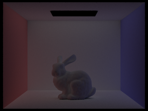
Here, you can really see that as we increase the number of samples per pixel, we begin to converge on the "real" image in our render. As we converge, we also minimize a lot of the noise.
So, noise can be eliminated by increasing the number of samples per pixel. What can we do with that information?
Part 5: Adaptive Sampling
What is Adaptive Sampling?
As we just saw, increasing the number of samples per pixel is good to reduce noise. But it also increases render time. Currently, we are sampling equally per pixel. But not all pixels were created equal; why sample 1024 times at a pixel that renders nothing?
Adaptive sampling remedies this issue, by keeping track of whether or not a pixel's radiance converges per sample.
Walkthrough
Our implementation is basically just a bunch of math, as specified
on the spec. To implement adaptive sampling, we will change the way
we sample in PathTracer::raytrace_pixel.
We first define all the variables we need.
float s1 = 0; // sum over radiance
float s2 = 0; // sum over radiance squared
int n = 0; // sample count
float mu = 0; // mean
float I = 0;
float sig2 = 0; // standard deviation
The formulae for these variables are given in the spec:* \[s_1 = \sum_{k=1}^n x_k, \quad s_2 = \sum_{k=1}^n x_{k}^2, \quad \mu = \frac{s_1}{n}, \quad \sigma^2 = \frac{1}{n - 1} \cdot \left(s_2 - \frac{s_1^2}{n}\right)\] \[I = 1.96 \cdot \sqrt{\frac{\sigma^2}{n}}\]
We're going to keep sampling until we meet our convergence critera (or hit the maximum number of samples):*
\[I \leq \text{maxTolerance} \cdot \mu\]
Additionally, to save some time, we are not checking convergence per sample taken;
we are given variable samplesPerBatch. In code, that looks like:
do {
    for (int i = 0; i < samplesPerBatch && n < num_samples; i++) {
        n += 1;

        ... // make ray

        Vector3D radiance = est_radiance_global_illumination(ray);
        average += radiance;
        float x_k = radiance.illum();
        s1 += x_k;
        s2 += x_k * x_k;
    }
    ... // calculate mu, sig2, I
} while (I > maxTolerance * mu && n < ns_aa);
Then we average over n samples and send to buffer like before.
Adaptive Sampling in Action
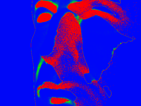
(The images were rendered at 2048 samples per pixel, 1 ray sample per light, and max ray depth 5 with Russian Roulette factor 0.35)
Note the red areas are sampled more, and the blue areas are sampled less. Red areas are covered in shadow, and blue areas are the background or directly lit spots.
AI Acknowledgement
For this homework, I used ChatGPT to help me format image tables on the write-up to have better spacing, layout, etc. ChatGPT did not generate any of the written text. Shout out to House M.D. Season 6 Episode 7 for giving me the inspiration to figure out global illumination. -Walter
Claude AI was utilized to debug Part 3, Task 3: Direct Sampling using Uniform Hemisphere Sampling. Bunny images were originally taking a humongous 17 minute time to render. -Crystal